Bayesian optimization with Gaussian process

Jun 29, 2022

Recently, I came across a paper on enzyme activity optimization using Bayesian optimization. I was fascinated at how efficient it is in saving time and lab resources in finding the optimal solution.

Why use it and when to use it?

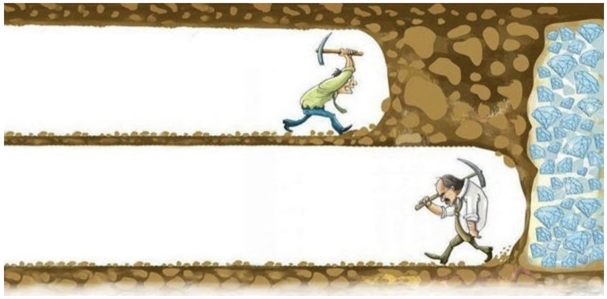
I’m going to borrow the example from Apoorv Agnihotri et.al on gold mining - imagine there is a piece of land with gold, you want to find the location with the highest gold content with minimum drilling.

This task satisfied the followings:

Find the global optima in the finite space (find the highest gold content location on a given land)
We don’t know or it’s expensive to learn the distribution of the underlying functions to optimize (drilling is expensive)
Want to minimize the number of experiments for finding the optima (drill as few times as possible)
The optimization procedure does not generally leverage derivative information (No plan to identify the location to drill based on the gold content change over locations - though one paper from NIPS 2017 explored Bayesian optimization with gradients)

Part I - Bayesian optimization

Bayesian optimization first treats the black box function f(x) (e.g gold content distribution) as a random function, we need a surrogate model (discussed in the part II below) that is flexible enough to model this random function as a probability distribution, such that we are not fitting the data to one known function but a collection of functions.

Because the black box function is modeled as a probability distribution, the Probability( gold content of a random location GIVEN f(gold content at known locations) AND a random location ) can be computed.

The prior distribution of f(x) can be derived from experience or with limited data points (e.g gold is usually distributed in the center of the land).

If this is the first round of the optimization, the limited gold content data points might come from drilling at random places, these data points are used to update the surrogate model to form the posterior distribution. An acquisition function further evaluates such posterior distribution to determine the most likely place to drill. For n th round of optimization, the data points will come from experimentally validated query points suggested by the acquisition function (e.g our acquisition function tells us 5 locations to drill, we drill the locations and use the gold content info from these 5 locations to update the prior model).

After we plug in the data points to the probability distribution setup from our assumptions/approximations, we get a conditional distribution over the value of the black-box function. We next use an acquisition function alpha(x) to determine how we select the next point to sample. The acquisition function is typically inexpensive that can be evaluated at a given point. There are several acquisition functions to choose from for balancing trade-offs between exploitation (focusing on sampling around current best values with low uncertainties) and exploration (searching for high variance and unexplored regions to discover potentially better results). Different acquisition functions give different strategies on selecting the next point to drill, but eventually, they will converge. It’s important to know that once an acquisition function is selected, one will stick with it through the course of the optimization.

Some popular acquisition functions:

Probability of improvement (PI): choose the next point as the one with the highest probability of improvements over the current best (doesn’t care about the amount of improvement). Occasionally, one might be stuck in local optima instead of global optima since the amount of improvement is not taken into account.

Expected improvement (EI): choose the next point as the one with the biggest improvements over the current max - it has two components, can be a location x where the expected value is the highest compared with the current best (exploitation), or can be a location x where with high uncertainty (exploration).

Upper confidence bound (UBC): choose the next point as the one with the highest expected value and uncertainty.

Part II - Gaussian process

In Bayesian optimization, we need a probabilistic model (also called a surrogate model) to approximate the black-box function.

The Gaussian process is frequently used as the surrogate model, given it is a random process where each point x (e.g location of the land) is assigned a random variable f(x) (e.g the gold content of the location x), and its joint distribution of a finite number of these variables p(f(x1), f(x2)…f(xn)) is also Gaussian. Gaussian distribution has many properties. The following slides are taken from Dr. Richard E. Turner.

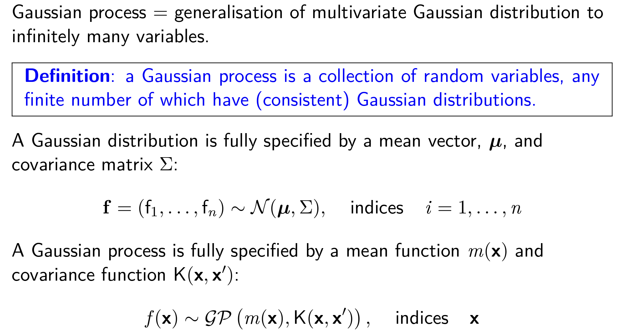
In a parametric model, a collection of parameters (e.g thetas) defines the model. The Gaussian process is a non-parametric model, wherein the non-parametric model, the number of parameters depends on the data size, since the covariance matrix is determined by the Gaussian radial basis function K(x1,x2) and noise (sigma_y), the dimension of the Gaussian radial basis function grows with data.

There are several parameters of the underlying Gaussian distribution that determines the shape of distribution of the black-box functions that Gaussian process is trying to infer. the l in the kernel function controls the level of wiggliness of the curve, the bigger the l, the more correlated nearby points are, and the less wiggly the curve will be when sampling from this kernel function.

Knowing that a Gaussian process samples from a multivariate Gaussian distribution, we can think of the problem as predicting the conditional probability distribution of unknown gold content given known data points and the relationship between known data points and unknown data points. See below.

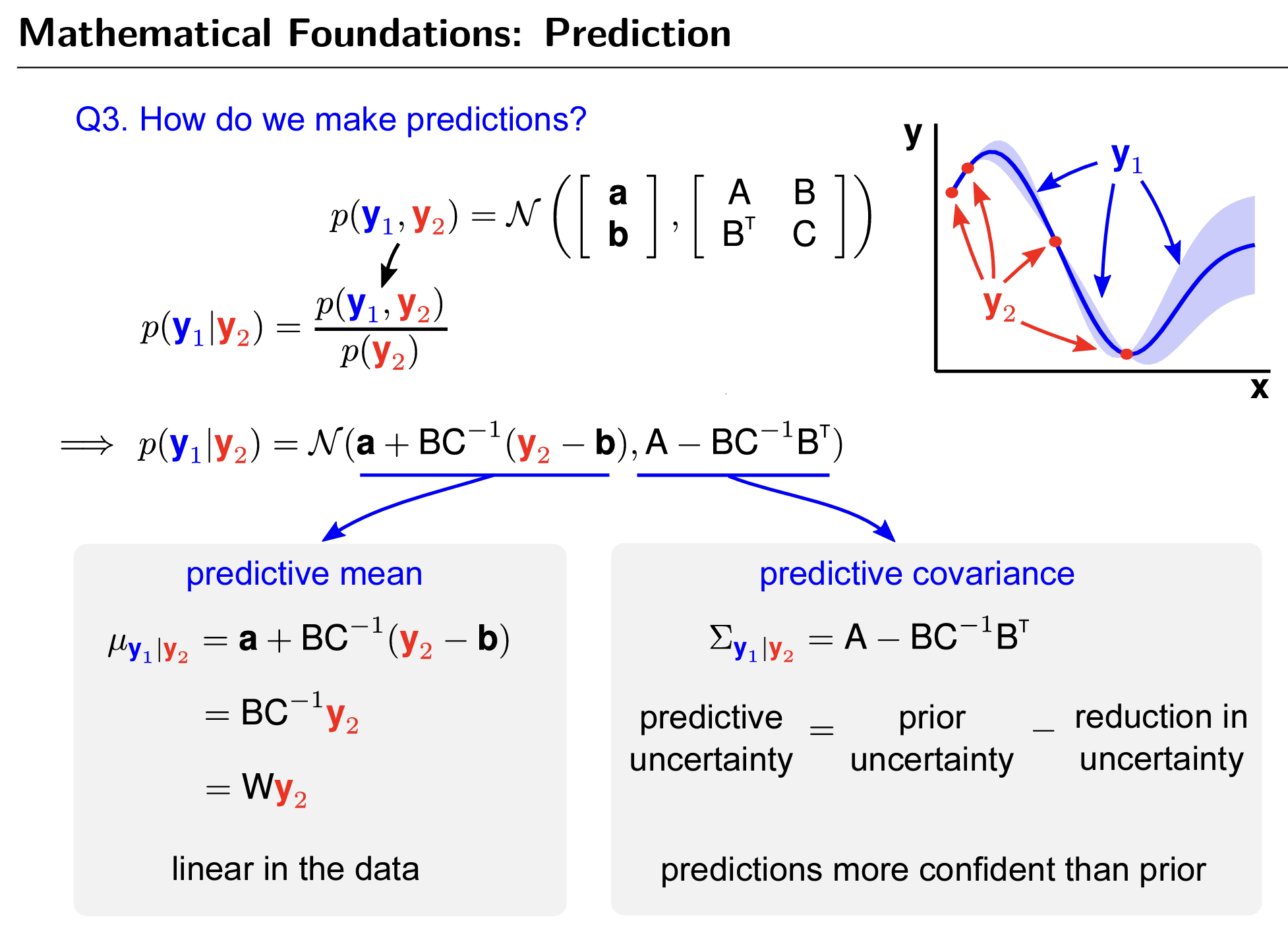
C indicates the covariance of training data (y2), while B indicates the covariance between predictive data points (y1) to training data (y2), and A is the covariance of predictive data points.

In order to predict the potential values in the unknown location with well-calibrated uncertainty, we plug in the values of the observed data as the prior over the underlying functions according to experience, it returns the posterior distribution over the underlying functions as well as the likelihood of the distribution parameters to be selected by acquisition function.

How to set the value of parameters in the Gaussian process

For the non-parametric model, we need to define kernel parameter l (to control the amount of correlation between data points), kernel parameter sigma (to control the vertical scale of the distribution), and noise parameter sigma_y. Such parameters are set in the 1st round of optimization and hold constant, but how to decide what numbers to use for these parameters?

It turns out that we can either do parameter tunning in the first round of model fitting (if we have enough data) and hold them constant in the following rounds of optimization or do retrospective studies once we collect enough data after n rounds(in this case the analysis is done post hoc). See Effect of kernel parameters and noise parameter section from Gaussian Process by Martin Krasser.

GPytorch, an efficient implmentation of Gaussian process in Pytorch also provides utilities to use gradient decent to optimize negative marginal log likelihood for the optimal parameters.

Q: How many rounds does it take to find the optima solution (e.g the highest gold content location) and how do we know we have it ??

The number of rounds of needed to do Bayesian optimization depend on the level of noise in the data, the accuracy of the prior assumptions, the area of the finite space to sample from. The paper on enzyme activity optimization had ~4,500 unique sequences to search from, and it took 9 rounds (each round <10 sequences were evaluated) of optimization to find the best performing enzyme. Instead of having to evalucate ~4,500 sequences in the lab one by one, the authors only needed to evaluate 90 sequences, that reduced the lab work to 2%!

Like other machine learning methods, the optima is reached either when we have learned the black-box functoin well enough (we drilled all possible locations on a given land) or we have found a satisfying answer within the budget.

Pros and Cons of Gaussian process from Dr. Richard E. Turner

Pros:

Probabilistic: one gets well-calibrated predictive uncertainty (e.g confidence interval) for decision making - neural networks do not provide
GP model is very generalized to even fit small data
Non-parametric: has an infinite-dimensional set of parameters with the capacity to learn from the training data

Cons:

GP is a single layer that doesn’t further infer complex hierarchical relationships between data points (can be solved by using a deep Gaussian process)
GP can be computationally expensive if we have many training samples.

When to not use Gaussian process

Given the formula of solving the conditional probability of the predicted points involves inverting the covariance matrix C of observed data (let’s say we have n observed samples so the covariance matrix C is a n x n matrix, the cost of doing the matrix inversion is x³). One way to work around this limitation is to summarize the n sample with m pseudo data points, where the m pseudo data points are selected to capture the real distribution of n data points (e.g fit a local Gaussian regionally with boundaries agreeing to each other).

GPytorch shows a smart implementation for using GP on big dataset.

Acknowledgement

I want to thank my friend Cihan Soylu for giving me an initial lecture on Bayesian optimization and for providing valuable feedbacks on the previous draft of this blog post. I also want to thank Alok Saldanda for suggesting wording revisions to this blog post.

Jiayi Wu Cox