A quick comparison between L1-LASSO and linear SVM
Recently I’ve been working on human lifestyle data to predict a certain disease. I have nearly ~4000 variables and would like to narrow down to a group of essential variables for the disease prediction. This process is called ‘feature selection’ in machine learning.
I tried using both L1-LASSO( least absolute shrinkage and selection operator) and linear SVM ( support vector machine) and got very similar result. L1-LASSO is the least square regression with L1 regularization, since the input variables are correlated, this method (unlike L2-norm ridge regression or somewhere between L1-L2 elastic net) will drop the highly correlated features rather than preserve every one of them. Linear SVM is a simplest classification algorithm using SVM without using any kernel tricks.
Now let’s compare the objective function in these two methods:
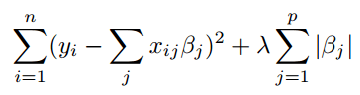
For L1-LASSO, we want to minimize the following, where lambda is the shrinkage factor (penalty) that applies to all the variables. Since we need to minimize the sum of square loss and L1 norm of betas, LASSO will find the balance using lambda. Big lambda (big penalty) will force some coefficients to be 0 and leave fewer variables in the model and vise versa.
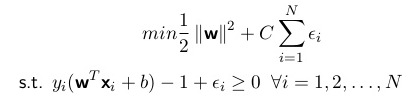
For linear SVM with soft margin (same formula for hard margin, can think of cost C as infinitely big), we are essentially minimizing the sum of the margin of each variable with a cost penalty. Similarly as L1-LASSO, epsilon will be computed automatically when given a fixed cost (shrinkage factor).
As you can see, the objective functions have very similar forms between L1-LASSO and linear SVM. Both methods can be done in R or in Python if you want to try it out, I use R more often but I strongly recommend Python scikit-learn package at least for SVM. With scikit-learn you can easily assemble your code without worrying about not being able to track the process hidden behind the scenes, more flexibility and complexity can also be used with Python.
Code to try in R
library(glmnet)

#build model with already standardized data
x_train<- model.matrix(~ ., train[,1:4000])
y_train<-train$outcome

#find lambda using 10 fold CV
cv.i<-cv.glmnet(x_train, y_train, nfold=10, family="binomial",type.measure="auc", keep =T, alpha=1, standardize=F,parallel=T)

# get lambdas
cv.i$lambda.min

# train the whole model with best lambda
predict.train<-glmnet(x_train, y_train, family="binomial", alpha=1, standardize=F, lambda= cv.i$lambda.min)

# apply trained model on test set
predict.test<-predict(predict.train, x_test, type="response")
Code to try in Python
import numpy as np
import pandas as pd
from sklearn.model_selection import GridSearchCV
from sklearn.svm import SVC

C=np.logspace(-20,15, base=2, endpoint=True, num=50 )
tuned_parameters =[{'kernel':['linear'], 'C':C}]
svm = SVC(C, kernel="linear", cache_size=1000, class_weight='balanced', probability=False)

# gridsearch with 10 CV for best C
clf = GridSearchCV(svm, tuned_parameters, cv=10,scoring='roc_auc',return_train_score=False )
clf.fit(x_train, y_train)

# print out the best parameters on training set
print("best score (best mean cv score of the best estimator)", clf.best_score_)
print("best paramerter", clf.best_params_)

# use the best C picked from training
C= clf.best_params_

#apply best C and run on test set
svm = SVC(C, kernel="linear", cache_size=1000, class_weight='balanced', probability=False)

svm_result = svm.fit(x_test, y_test)